 Hi
Hi
I sense that a lot of people are looking for a simple triangulation method with OpenCV, when they have two images and matching features.
While OpenCV contains the function cvTriangulatePoints in the triangulation.cpp file, it is not documented, and uses the arcane C API.
Luckily, Hartley and Zisserman describe in their excellent book “Multiple View Geometry” (in many cases considered to be “The Bible” of 3D reconstruction), a simple method for linear triangulation. This method is actually discussed earlier in Hartley’s article “Triangulation“.
I implemented it using the new OpenCV 2.3+ C++ API, which makes it super easy, and here it is before you.
Edit (4/25/2015): In a new post I am using OpenCV’s cv::triangulatePoints() function. The code is available online in a gist.
Edit (6/5/2014): See some of my more recent work on structure from motion in this post on SfM and that post on the recent Qt GUI and SfM library.
Update 2017: See the new Mastering OpenCV3 book with a deeper discussion, and a more recent post on the implications of using OpenCV3 for SfM.
The thing about triangulation is that you need to know the extrinsic parameters of your cameras – the difference in location and rotation between them.
To get the camera matrices… that’s a different story that I’m going to cover shortly in a tutorial (already in writing) about Structure from Motion.
But let’s assume that we already have the extrinsic matrices. In most cases, where you know what the motion is (you took the pictures :), you can just write the matrices explicitly.
Linear Triangulation
/**
 From "Triangulation", Hartley, R.I. and Sturm, P., Computer vision and image understanding, 1997
 */
Mat_ LinearLSTriangulation(Point3d u,		//homogenous image point (u,v,1)
				   Matx34d P,		//camera 1 matrix
				   Point3d u1,		//homogenous image point in 2nd camera
				   Matx34d P1		//camera 2 matrix
								   )
{
	//build matrix A for homogenous equation system Ax = 0
	//assume X = (x,y,z,1), for Linear-LS method
	//which turns it into a AX = B system, where A is 4x3, X is 3x1 and B is 4x1
	Matx43d A(u.x*P(2,0)-P(0,0),	u.x*P(2,1)-P(0,1),		u.x*P(2,2)-P(0,2),
		  u.y*P(2,0)-P(1,0),	u.y*P(2,1)-P(1,1),		u.y*P(2,2)-P(1,2),
		  u1.x*P1(2,0)-P1(0,0), u1.x*P1(2,1)-P1(0,1),	u1.x*P1(2,2)-P1(0,2),
		  u1.y*P1(2,0)-P1(1,0), u1.y*P1(2,1)-P1(1,1),	u1.y*P1(2,2)-P1(1,2)
			  );
	Mat_ B = (Mat_(4,1) <<	-(u.x*P(2,3)	-P(0,3)),
					  -(u.y*P(2,3)	-P(1,3)),
					  -(u1.x*P1(2,3)	-P1(0,3)),
					  -(u1.y*P1(2,3)	-P1(1,3)));
	Mat_ X;
	solve(A,B,X,DECOMP_SVD);
	return X;
}
This method relies very simply on the principle that every 2D point in image plane coordinates is a projection of the real 3D point. So if you have two views, you can set up an overdetermined linear equation system to solve for the 3D position.
See how simple defining a Matx43d struct from scratch and using it in solve(..) is?
I tried doing some more fancy stuff with Mat.row(i) and Mat.col(i), trying to stick to Hartley’s description of the A matrix, but it just didn’t work.
Using it
Using this method is easy:
//Triagulate points
void TriangulatePoints(const vector& pt_set1,
					   const vector& pt_set2,
					   const Mat& Kinv,
					   const Matx34d& P,
					   const Matx34d& P1,
					   vector& pointcloud,
					   vector& correspImg1Pt)
{
#ifdef __SFM__DEBUG__
	vector depths;
#endif
	pointcloud.clear();
	correspImg1Pt.clear();
	cout << "Triangulating...";
	double t = getTickCount();
	unsigned int pts_size = pt_set1.size();
#pragma omp parallel for
	for (unsigned int i=0; i		Point2f kp = pt_set1[i];
		Point3d u(kp.x,kp.y,1.0);
		Mat_ um = Kinv * Mat_(u);
		u = um.at(0);
		Point2f kp1 = pt_set2[i];
		Point3d u1(kp1.x,kp1.y,1.0);
		Mat_ um1 = Kinv * Mat_(u1);
		u1 = um1.at(0);
		Mat_ X = IterativeLinearLSTriangulation(u,P,u1,P1);
//		if(X(2) > 6 || X(2) < 0) continue;
#pragma omp critical
		{
			pointcloud.push_back(Point3d(X(0),X(1),X(2)));
			correspImg1Pt.push_back(pt_set1[i]);
#ifdef __SFM__DEBUG__
			depths.push_back(X(2));
#endif
		}
	}
	t = ((double)getTickCount() - t)/getTickFrequency();
	cout << "Done. ("<
	//show "range image"
#ifdef __SFM__DEBUG__
	{
		double minVal,maxVal;
		minMaxLoc(depths, &minVal, &maxVal);
		Mat tmp(240,320,CV_8UC3); //cvtColor(img_1_orig, tmp, CV_BGR2HSV);
		for (unsigned int i=0; i			double _d = MAX(MIN((pointcloud[i].z-minVal)/(maxVal-minVal),1.0),0.0);
			circle(tmp, correspImg1Pt[i], 1, Scalar(255 * (1.0-(_d)),255,255), CV_FILLED);
		}
		cvtColor(tmp, tmp, CV_HSV2BGR);
		imshow("out", tmp);
		waitKey(0);
		destroyWindow("out");
	}
#endif
}
Note that you must have the camera matrix K (a 3×3 matrix of the intrinsic parameters), or rather it’s inverse, noted here as Kinv.
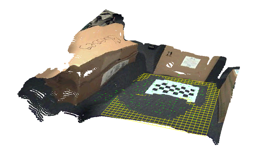
Results and some discussion


Notice how stuff is distorted in the 3D view… but this is not due projective ambiguity! as I am using the Essential Matrix to obtain the camera P matrices (cameras are calibrated). Hartley and Zisserman explain this in their book on page 258, and the reasons for projective ambiguity (and how to resolve it) on page 265. The distortion must be due to inaccurate point correspondence…
The cool visualization is done using the excellent PCL library.
Iterative Linear Triangulation
Hartley, in his article “Triangulation” describes another triangulation algorithm, an iterative one, which he reports to “perform substantially better than the […] non-iterative linear methods”. It is, again, very easy to implement, and here it is:
/**
 From "Triangulation", Hartley, R.I. and Sturm, P., Computer vision and image understanding, 1997
 */
Mat_<double> IterativeLinearLSTriangulation(Point3d u,	//homogenous image point (u,v,1)
											Matx34d P,			//camera 1 matrix
											Point3d u1,			//homogenous image point in 2nd camera
											Matx34d P1			//camera 2 matrix
											) {
	double wi = 1, wi1 = 1;
	Mat_<double> X(4,1);
	for (int i=0; i<10; i++) { //Hartley suggests 10 iterations at most
		Mat_<double> X_ = LinearLSTriangulation(u,P,u1,P1);
		X(0) = X_(0); X(1) = X_(1); X(2) = X_(2); X_(3) = 1.0;
		//recalculate weights
		double p2x = Mat_<double>(Mat_<double>(P).row(2)*X)(0);
		double p2x1 = Mat_<double>(Mat_<double>(P1).row(2)*X)(0);
		//breaking point
		if(fabsf(wi - p2x) <= EPSILON && fabsf(wi1 - p2x1) <= EPSILON) break;
		wi = p2x;
		wi1 = p2x1;
		//reweight equations and solve
		Matx43d A((u.x*P(2,0)-P(0,0))/wi,		(u.x*P(2,1)-P(0,1))/wi,			(u.x*P(2,2)-P(0,2))/wi,
				  (u.y*P(2,0)-P(1,0))/wi,		(u.y*P(2,1)-P(1,1))/wi,			(u.y*P(2,2)-P(1,2))/wi,
				  (u1.x*P1(2,0)-P1(0,0))/wi1,	(u1.x*P1(2,1)-P1(0,1))/wi1,		(u1.x*P1(2,2)-P1(0,2))/wi1,
				  (u1.y*P1(2,0)-P1(1,0))/wi1,	(u1.y*P1(2,1)-P1(1,1))/wi1,		(u1.y*P1(2,2)-P1(1,2))/wi1
				  );
		Mat_<double> B = (Mat_<double>(4,1) <<	-(u.x*P(2,3)	-P(0,3))/wi,
						  -(u.y*P(2,3)	-P(1,3))/wi,
						  -(u1.x*P1(2,3)	-P1(0,3))/wi1,
						  -(u1.y*P1(2,3)	-P1(1,3))/wi1
						  );
		solve(A,B,X_,DECOMP_SVD);
		X(0) = X_(0); X(1) = X_(1); X(2) = X_(2); X_(3) = 1.0;
	}
	return X;
}
(remember to define your EPSILON)
This time he works iteratively in order to minimize the reprojection error of the reconstructed point to the original image coordinate, by weighting the linear equation system.
Recap
So we’ve seen how easy it is to implement these triangulation methods using OpenCV’s nice Matx### and Mat_
Also solve(…,DECOMP_SVD) is very handy for overdetermined non-homogeneous linear equation systems.
Watch out for my Structure from Motion tutorial coming up, which will be all about using OpenCV to get point correspondence from pairs of images, obtaining camera matrices and recovering dense depth.
If you are looking for more robust solutions for SfM and 3D reconstructions, see:
http://phototour.cs.washington.edu/bundler/
http://code.google.com/p/libmv/
http://www.cs.washington.edu/homes/ccwu/vsfm/
Enjoy,
Roy.
46 replies on “Simple triangulation with OpenCV from Harley & Zisserman [w/ code]”
Hello, Roy.
I am new in Computer Vision and I found your tutorial is really useful. I have just one question. I have stereo camera system. I calibrated my stereo system. What I want to do is: if I have some 2D points of the image from left camera, how could I found out what are 3D coordinates of those points in the space relative to the left camera?
Thank you.
@Ban
In your case you do not need a Sturcture from Motion method, but rather a stereo rig calibration method.
There are many functions in OpenCV to support that, and even some very simple tools
Check out
https://code.ros.org/svn/opencv/trunk/opencv/samples/cpp/stereo_calib.cpp
https://code.ros.org/svn/opencv/trunk/opencv/samples/cpp/stereo_match.cpp
Using these methods will end up with a disparity map, and even a point cloud!
hi, Roy:
It seems i can not send email to you by the email you post on the website. Anyway, I have question about the post https://www.morethantechnical.com/2010/03/06/implementing-ptam-stereo-tracking-and-pose-estimation-for-ar-with-opencv-w-code/.
In your code, you used [R|T] as the projection matrix, however, I think it should be K[R|T], where K is the intrinsic matrix. Could you tell me the reason, or I misunderstand something here. Thanks!!!
@Hover
If you look carefully at the code, you’ll see I am using undistortPoints(…), which converts them already to their canonical form and corrects the radial distortion.
So all the 2D points are already corrected, no need to use the K matrix.
However that post is somewhat outdated.
Look out for a new post (very) soon about structure from motion and camera pose estimation.
hi, Roy:
Thanks for your reply. So, it means the undistort(srcImg, dstImg, …) and undistortPoints(srcPts, dstPts, …) is different, right? The dstPts from undistortPoints() is K_inverse * undistorted_srcPts, while the dstImg from undistort() is undistored_srcImg. Is it right?
Thanks!
Hi Rob,
Thank you for all the invaluable experience that you share in your posts, it helps and inspires me a lot!
I’ve still a question though. I guess from your screenshots that you’re working on a Mac, as I am. I’m trying to use PCL to display my own results of 3D reconstruction, but I can’t get PCL to work correctly. Could you please share some hints or tips on how you installed and ran PCL on your machine (even very briefly) ?
Again, thanks a lot.
@Emmanuel
For making PCL work on the mac, what did the trick for me was to compile VTK to use X11 instead of Cocoa.
PCL relies on VTK for visualization, and I just couldn’t make it work using Cocoa… but X11 works perfect.
@Rob
Thanks for the answer. I’ll try to install VTK from macports then, to have easy X11 support, since the binary VTK package from PCL seems to be missing a few things (libXt.dylib at least, for me).
Hi
Nice tutorial.
You mentioned that Mat.row() and mat.col didnt work for you…this seems to work for me..let us cross check.
Also since “solve” involves an inverse it is much more expensive I believe.
Mat compute_LinearTriangulation(const Mat & ProjMat1, const Mat & points1 , const Mat & ProjMat2, const Mat & points2)
{
Mat A(4,4,CV_64F),U,V,S,X3D(4,points1.rows,CV_64F);
for (int i=0;i<points1.rows;i++){
A.row(0)=points1.at(i,0)*ProjMat1.row(2)-ProjMat1.row(0);
A.row(1)=points1.at(i,1)*ProjMat1.row(2)-ProjMat1.row(1);
A.row(2)=points2.at(i,0)*ProjMat2.row(2)-ProjMat2.row(0);
A.row(3)=points2.at(i,1)*ProjMat2.row(2)-ProjMat2.row(1);
SVD::compute(A,S,U,V);
X3D.col(i)=V.t().col(3)/V.at(4,4);
}
return X3D;
}
regards
Daniel
*edit everywhere..my bad
points1.at(i,0~1)
hey roy,
thanks for your nice tutorial.
But there are some errors in your code.
In “IterativeLinearLSTriangulation”:
* X_(3) = 1.0; change to X(3) = 1.0;
* the iteration make no sense, because no involved parameter
is changing, so your “fabsf(wi – p2x)” is zero and nothing happends.
cheers
Marc
=> edit:
* you have to set
cv::Mat_ X_ = LinearLSTriangulation(u,P,u1,P1);
X(0) = X_(0); X(1) = X_(1); X(2) = X_(2); X(3) = 1.0;
before the loop
@Marc
Thank you for the correction! I changed the code.
Hi Rob,
How do you get the Matx34d P and Matx34d P1 camera matrices?
If you have calibrated stereo cameras, I guess the P matrix of the reference camera is just its K matrix and the other P matrix is egal to [K1R|-K1Rt]?
Thx in advance for your help!
@Jean-Philippe
I get the P matrices from the fundamental matrix (actually the essential matrix, using the K calibration matrix).
In a calibrated stereo pair indeed you have the R and t components discovered during the calibration process…
Roy,
Thx for your answer! Actually my question should have been more precise: I have a calibrated video rig, so I got the K matrix (intrinsics camera parameters) for each camera as well as the R and t components (extrinsic parameters of the rig). Having that how should I properly build the P and P1 matrices in order to feed your fonctions? Is P = K (for the left camera) and P1 = [K1R|-K1Rt] (assuming K1 the K matrix of the right camera)?
Again, thx in advance for your help!
@Jean-Phillipe
Basically one camera you can keep as P=[I|0] (identity rotation and 0 translation), and the other camera P=[R|t]
When you want to triangulate (you have point matches pairs represented in pixel coordinates) you can simply multiply them by K and then triangulate.
Indeed you may left-multiply the P by the respective K to save on some time. But first check by debugging that the values make sense
Hello Roy,
My research needs to do experiment using 4 cameras to get simultaneous multi-images. So, I want to get mapping function to do the 3d reconstruction but I am new in computer vision. May you recommend me a tool to set up the calibration with these multiple cameras!?
hi Roy,
i think your source code is buggy at file Triangulation.cpp line 71 to 97 (watched at github). First you call the linear triangualtion method and after that you reweight the A and B matrix to calculate X again. Thats good but at line 71 you call the linear triangualtion method again, that overwrites the previous calculation of X. At the end each iteration ends with i == 1. Did i missunderstand your source code???
Thx in advance for your help!
Hi Roy,
I have camera mounted on robot hand. I have Intrinsic camera parameters, known position of camera in robot coordinate system, and pxel coordinate point on both images. How compute u, v , P1 , P2 ?
@Slava
If you have the position of the robot – you basicaly have P1 and P2
Just put the position (translation/movement, and rotation) in an P = [R|t] matrix form, and then triangulate.
u and v are simply the pixel coordinated. you can either take a pixel (x,y,1) and multiply by K (intrinsics) or leave it (x,y,1) and use the K*P1 matrix (intrinsics multiplied by your camera positiong matrix).
Hi Roy,
Is the whole project code (also with data) available in the svn repository? (I mean, http://code.google.com/p/morethantechnical/)
I would like to replicate your result from the data.
Thanks in advance!
Dear Roy,
I notice that in your code you set the homogeneous part of 3D output points equals to 1. However how do you manage noisy points that may have negative depth ? Or points at infinity ? Shouldn’t you set the homogeneous part to 0 in these cases, based on the depth of the 3D points ?
@Guido,
Indeed this is a strong assumption on the reconstructed scene.
But I am really looking only for points that are forward of the cameras (or else they would not be visible in the images), and points on the infinite plane are no good for recovering motion…
Points that will be too far from the originating 2D position will be removed .
Dear Roy,
To reconstruct 3d points, Can I use this code using correspondence points of moving object in two different image sequence from single stationary camera. In my case, how to use camera calibration matrix (K)?
Hi Roy,
I have a stereo rigged which is calibrated. I use P = (I|O) for my first camera and P = Extrinsic (R|T) for my second.
Both images are already undistorted using the Undistort function of OpenCV (or EmguCV rather, since I work in C# .Net).
Anyway, when I use your code, to determine the distance between 2 points, it goes berserk! I use the basic Pythogaron way to determine distance (dist = sqrt(dx^2 + dy^2 + dz^2), which should work as far as I’m concerned.
The points I try to find are the first and last corner of my 8×6 checkerboard, using findCheckerboardCorners, so they should be relatively stable, but when I move the checkerboard around, the numbers change constantly.
Can you help?
Thank you very much in advance.
Regards,
Michael
[…] implemented the linear triangulation methods they present, and wrote a post about it not long ago: Here. I also added the Iterative Least Squares method that Hartley presented in his article […]
Hi Roy – I am trying to triangulate points….
I have 2 calibrated cameras, which I then use OpenCVs StereoRectify to produce 2 ‘virtual’ cameras with the y (or v) co-ordinates equal.
I then use my own method to find correspondences.
From StereoRectify I have P1 and P2 (3×4 projection matrices, which look like camera intrinsic matrices plus an extra righthand column for ?translation)
Are these the same as your P1 and P2 ? If so, what should I use for K (or KInv?). I have the original R and T, and R1 and R2 (returned from StereoRectify) which are the rotations of the ‘virtual’ cameras. Bear in mind my correspondences are in the Rectified images.
Any ideas how to proceed ?
hi Roy,
Great code, great example.
I still am wondering about the “bugs” Marc posted a year ago.
In the IterativeLinearLSTriangulation() function I cant see any update in the values, so it always exits in the second loop. nor u,P,u1,or P1 changes in the loop so LinearLSTriangulation() returns the same and the condition to exit the loop always is true. Stil I cant see what is needed to change. Any idea?
Hi Roy, thank you for your work.
I started studying computer vision quite recently, and I’ve a question about the linear system you want to solve.
I don’t understand why you define, and what it represents, the “B” matrix in your implementation. In “Multiple view geometry” (Zisserman) the linear triangulation method is defined using only the “A” matrix and solving the system AX=0 where X are the 3D coordinates. Can you please explain me?
Thanks!
very good tutorial for stereo vision with a powerful vision software like Opencv. I add a link of your article to my post about stereo vision systems uses in robotics, tutorials and resources
Thanks for sharing, nice piece of code. I see you are using some multi-threading, which will probably influence and concflict the timer you have build around your #pragma expression. (the gettickcount will probably not account for multiple processors, correct?).
Hi..
i have two motion capture cameras from Optitrack and i want to use them to track 3d position of a marker specialized for the camera.
I managed to get each of the camera to output 2d position of the marker.
Can i use the marker position from the cameras to triangulate it’s 3d position using this method? or are there a simpler solution? i dont have the camera matrices and i’m still unable to understand how to get the camera matrices using opencv.
thanks
Hello Roy,
First of all, very nice explanation. I’m new to computer vision but I’ve done a handheld code that takes to pictures, tracks the features and I created a disparity map from them, now I want to create a 3D representation out of it, probably a point cloud will be the easiest thing, using openCV, what else do I have to calculate and how do I create the point cloud? (trying to avoid PCL library but if it is really necessary I’ll use it).
Hi Roy,
just wanted to let you know that in the source code on this page there is the error mentioned by Marc where
X(0) = X_(0); X(1) = X_(1); X(2) = X_(2); X_(3) = 1.0;
should be
X(0) = X_(0); X(1) = X_(1); X(2) = X_(2); X(3) = 1.0;
There are two lines (!) where this need to be changed.
Best regards,
Chris
Hi, Thank you for your tutorial.
I read the Hartley’s article “Triangulation”. I dont know if my understanding is right, for the Iterative LS method, in your code:
Mat_ X_ = LinearLSTriangulation(u,P,u1,P1);
X(0) = X_(0); X(1) = X_(1); X(2) = X_(2); X(3) = 1.0;
This part of code should be outside the “for loop” as calculating the initial value for the 3D point (X).
Regards
Ping
Hello Sir roy,
I am very new in computer vision and just started learning some stuff. I have some aerail images from uav and I want to reconstruct 3D from it. Upto now i have taken a pair of image and have obtained feature matches from two images. Now what i need to do to get d point cloud from them. I am confused . Can you giove me answers.
Hello,Roy,
I do some research on 3D reconstruction recently,and I download your code called SfM-Toy-Library-master.I can not understand a funtion called TestTriangulation in your code .Why do you check for coplanarity of points in this function.That make me confused, Could you please give me some explaination?
Hi Roy,
I tried your algorithm but I can’t get the expected results.
I have 2 cameras and this parameters:
Cam1
Resolution: 2448 x 2050 pixels, Pixel Size = 0.0035 mm
c = 5.0220 mm
xp = 0.1275 mm
yp = 0.0453 mm
—————————————————————
Cam2
Resolution: 2448 x 2050 pixels, Pixel Size = 0.0035 mm
c = 5.0346 mm
xp = 0.0940 mm
yp = 0.0484 mm
And 2 images, one from cam1 and one from cam2
// Should be the translation
Camera Image Xc Yc Zc
# 1 cam1.jpg 0.0000 -0.0000 0.0000
# 2 cam2.jpg 982.4417 125.7794 82.7234
// Orientation matrices
Image R11 R12 R13 R21 R22 R23 R31 R32 R33
cam1.jpg 1.000000 0.000000 0.000000 0.000000 -0.000000 1.000000 0.000000 -1.000000 -0.000000
cam2.jpg 0.936824 0.337783 0.090899 -0.055027 -0.114315 0.991919 0.345445 -0.934256 -0.088506
Is that enough to run the process?
i tried something like this but I can’t get the expected result
Matx34d cam0(
1.000000, 0.000000, 0.000000, 0.000000,
0.000000, -0.000000, 1.000000, 0.000000,
0.000000, -1.000000, -0.000000, 0.000000
);
Matx34d cam1(
0.936824, 0.337783, 0.090899, 982.4417,
-0.055027, -0.114315, 0.991919, 125.7794,
0.345445, -0.934256, -0.088506, 82.7234
);
Point3d p1(1677, 360, 1);
Point3d p2(1684, 533, 1);
Mat_ result = IterativeLinearLSTriangulation(p1, cam0, p2, cam1);
Hi Roy, when you use Mat_ um for example, my compiler show me a bug, it have to be Mat_ um i think. On the other hand, the bugs that the people previosly talked about the code inside de loop, etc, are still in the post, can you fix it please ?
Thnks
Hi, if somebody have the triangulation method OK, please can send me at my email, i am begining in computer vision, and i have readed that the OpenCv triangulatePoints() method doesn’t work very precisely, because the method that is used inside.
Thanks.
@Jose
I’ve written a new blog post properly utilizing the cv::triangulatePoints function, see the function in the gist: https://gist.github.com/royshil/7087bc2560c581d443bc#file-simpleadhoctracker-cpp-L93
Hi, thanks a lot for the tutorial.
I have small doubt can you please say me.
What are
const vector& pt_set1,
const vector& pt_set2,
I didn’t get pt_set1 and pt_set2. From where these came ?
Please solve for me.
Regards
Suhas
Hi!
Can you help me?
I can’t understand this moment:
double p2x = Mat_(Mat_(P).row(2)*X)(0);
I have camera matrix P=[1 0 0 0;0 1 0 0;0 0 1 0] for the first image.
This equation is equal to zero, isn’t it?
Hi!
thanks for tutorial.
Is it possible to use this method to 3 or more views?
Hello,
I am new in Computer Vision and I found your tutorial is really useful. I have one question. I have stereo camera system and I have calibrated the system. I calculate P1 and P2 from K1, R and T. So i have P=[I|0] (identity rotation and 0 translation), and the other camera P=[R|t] and then i triangulate. But for a flat surface i must have constant depth values but i have depth “linear”, it could be due to fact that my cameras are tilted so as the origin of the landmark must be left camera and the depth axis direction is not normal to my surface? How to correct it? thanks for your help